---
title: "Top 500 Novels Metadata Analysis"
categories: [exercise, solution, python, rankings, correlations]
#image: "https://upload.wikimedia.org/wikipedia/commons/e/ed/US-Mexico_barrier_map.png"
format:
html: default
ipynb: default
code-overflow: wrap
code-fold: show
editor: visual
df-print: kable
R.options:
warn: false
code-tools: true
execute:
eval: true
---
# Metadata Analysis
### By Aashna Sheth
Let's start by reading our data into a pandas dataframe. A pandas dataframe is a structure used to hold file data. This structure has efficient methods used for manipulating and visualizing data.
```{python}
import matplotlib.pyplot as plt
import pandas as pd

df = pd.read_csv("https://raw.githubusercontent.com/melaniewalsh/responsible-datasets-in-context/refs/heads/main/datasets/top-500-novels/top-500-novels-metadata_2025-01-11.csv", sep=',', header=0, low_memory=False)
```
Now, we can answer various questions using this structure, which we've named `df`.
For example, let's look at counts related to author gender and name.
```{python}
#| colab: {base_uri: 'https://localhost:8080/', height: 209}
df["author_gender"].value_counts(dropna=False)
```
We see that about 70% of authors on the list are male and 30% are female.
Some authors appear multiple times on the list. Let's see which authors are most represented in the list.
```{python}
#| colab: {base_uri: 'https://localhost:8080/', height: 429}
df["author"].value_counts(dropna=False).head(10)
```
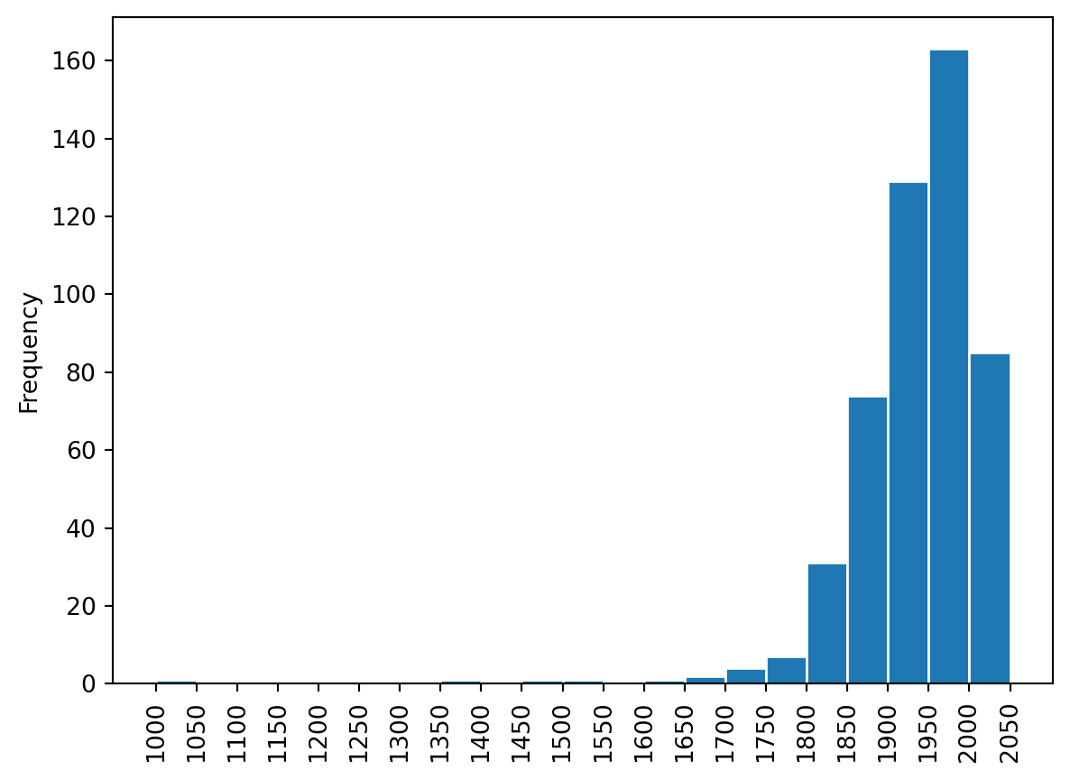
Next, we can delve into some visualization work to understand where authors are from and what timeframe of publication is most represented in the top 500 list.
```{python}
#| colab: {base_uri: 'https://localhost:8080/', height: 451}
import numpy as np

bins = np.arange(1000, 2060, 50)
bars = df['pub_year'].plot.hist(bins=bins, edgecolor='w')
plt.xticks(rotation='vertical');
plt.xticks(bins);
```
We can see that most books on the list were published between 1950 and 2000. Let's take a look at information about the oldest and newest books on the list.
```{python}
#| colab: {base_uri: 'https://localhost:8080/', height: 375}
from IPython.display import display

print("Oldest Book(s):")
display(df[df["pub_year"]==df["pub_year"].min()])
print("Newest Book(s):")
display(df[df["pub_year"]==df["pub_year"].max()])
```
Let's take a look at where the authors are from!
```{python}
#| colab: {base_uri: 'https://localhost:8080/', height: 272}
df["author_nationality"].value_counts().head(5)
```
---
Finally, let's unpack the differences between the Goodreads ratings and the top 500 ratings. First, we should think about how we want to compare the two lists. Given that we have listed rankings by average rating and number of ratings, which metric would be better to use? Would we want to create another metric?
For our purposes, we decided to use number of ratings, instead of average rating, as OCLC measures popularity by number of holdings, not how much patrons say they enjoy reading the books.
```{python}
#| colab: {base_uri: 'https://localhost:8080/'}
def top_5_comparison(col_name):
  print(df[["title", "author", "top_500_rank", col_name]].head(5))

  sorted = df.sort_values(by=[col_name])
  print(sorted[["title", "author", "top_500_rank", col_name]].head(5))

top_5_comparison("gr_num_ratings_rank")
```
Above you can see that the Goodreads rankings and the top 500 rankings aren't very aligned!
What factors affect popularity on Goodreads compared to OCLC?
```{python}
#| colab: {base_uri: 'https://localhost:8080/'}
import math

def print_rankings(d, col_name):
    rank_B = d[col_name]
    rank_A = d["top_500_rank"]
    title = d["title"]
    points_moved = 0
    if (math.isnan(rank_B)):
      points_moved = 501
    else:
      if rank_B > int(rank_A):
          points_moved = rank_B - rank_A
          print(f"\u001b[31m ▼ -{int(points_moved)} {title}")
      elif rank_B < rank_A:
          points_moved = rank_A - rank_B
          print(f"\u001b[32m ▲ +{int(points_moved)} {title}")
      else:
          print(f"\u001b[30m ● {int(points_moved)} {title}")
    d["points_moved"] = int(points_moved)
    return d

df = df.apply(lambda d: print_rankings(d, "gr_num_ratings_rank"), axis=1)
```
Let's see which novels had the most movement up or down!
```{python}
#| colab: {base_uri: 'https://localhost:8080/'}
sorted = df.sort_values(by=['points_moved'])
print(sorted[["title", "author", "points_moved", "top_500_rank", "gr_num_ratings_rank"]].head(10).to_string(index=False))
```
```{python}
#| colab: {base_uri: 'https://localhost:8080/'}
sorted = df.sort_values(by=['points_moved'], ascending=False)
print(sorted[["title", "author", "points_moved", "top_500_rank", "gr_num_ratings_rank"]].head(10).to_string(index=False))
```
Above we see that Steinbeck's "The Winter of Our Discontent", stayed at the same ranking of 397. Pride and Prejudice remained quite high as well.
20k Leagues under the sea dropped the most, from rank 37 in the top 500 list, to rank 481 in the goodreads list! Harry Potter and The Sea of Monsters rose up the most.
```{python}
#| colab: {base_uri: 'https://localhost:8080/'}
df['points_moved'].mean()
```
---
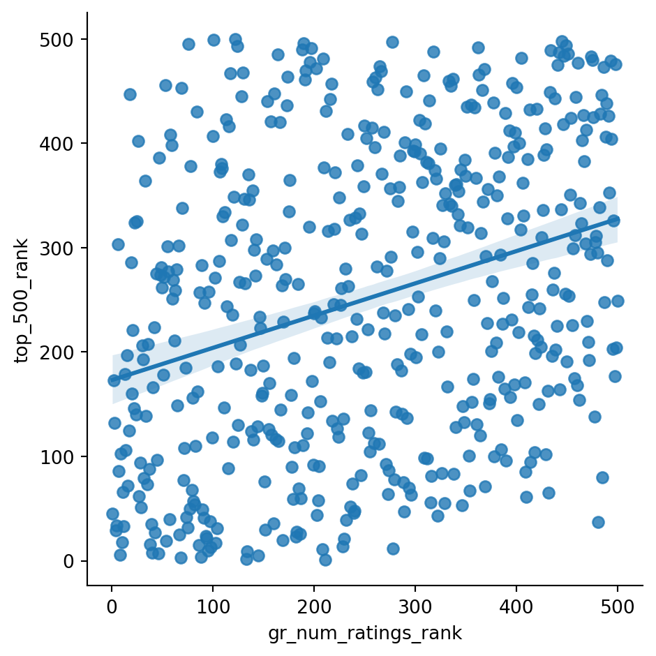
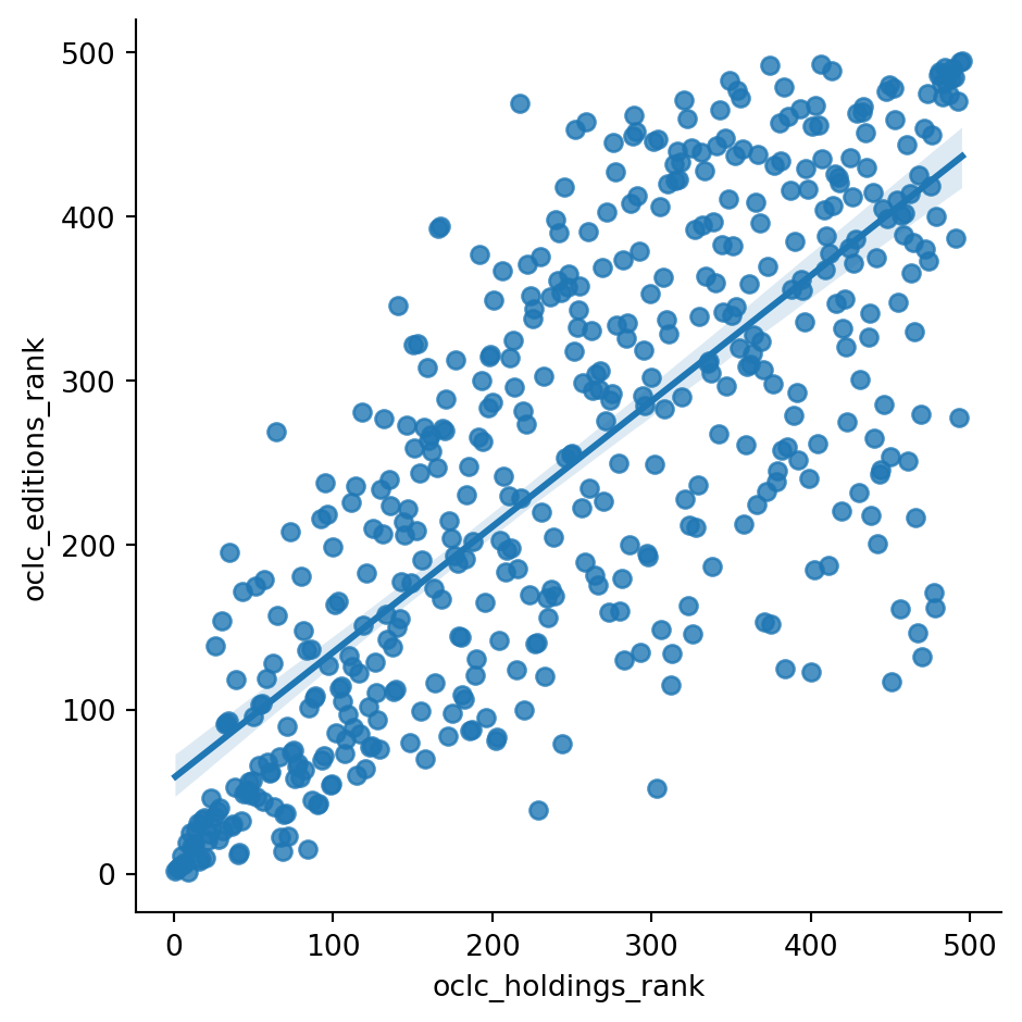
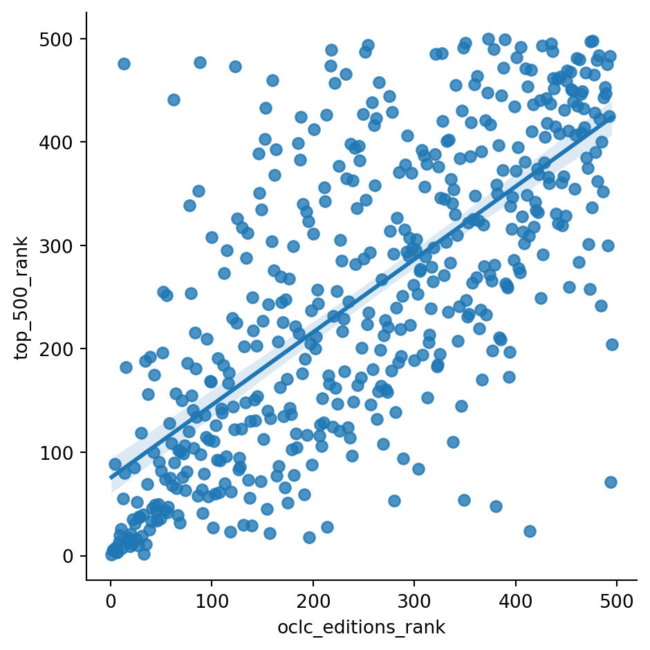
Let's take a look at some of these metrics for rankings based on number of editions and total holdings.
```{python}
#| colab: {base_uri: 'https://localhost:8080/', height: 1000}
import pandas as pd
import seaborn as sns
from scipy import stats
# inspired by: https://www.sfu.ca/~mjbrydon/tutorials/BAinPy/08_correlation.html

sns.lmplot(x="gr_num_ratings_rank", y="top_500_rank", data=df)
print(stats.pearsonr(df['gr_num_ratings_rank'], df['top_500_rank']))

sns.lmplot(x="oclc_holdings_rank", y="oclc_editions_rank", data=df)
dropped_df = df[df.oclc_editions_rank.notna() & df.oclc_holdings_rank.notna()]
print(stats.pearsonr(dropped_df['oclc_holdings_rank'], dropped_df['oclc_editions_rank']))

sns.lmplot(x="oclc_editions_rank", y="top_500_rank", data=df)
dropped_df = df[df.oclc_editions_rank.notna()]
print(stats.pearsonr(dropped_df['oclc_editions_rank'], dropped_df['top_500_rank']))
```
```{python}
#| colab: {base_uri: 'https://localhost:8080/'}
df = df.apply(lambda d: print_rankings(d, "oclc_editions_rank"), axis=1)
```
```{python}
#| colab: {base_uri: 'https://localhost:8080/'}
df = df[df["points_moved"] <= 500]
top_5_comparison("oclc_editions_rank")
```
```{python}
#| colab: {base_uri: 'https://localhost:8080/'}
df['points_moved'].mean()
smaller_df = df.head(10)
smaller_df['points_moved'].mean()
```
---
```{python}
#| colab: {base_uri: 'https://localhost:8080/'}
df = df.apply(lambda d: print_rankings(d, "oclc_holdings_rank"), axis=1)
```
```{python}
#| colab: {base_uri: 'https://localhost:8080/'}
top_5_comparison("oclc_holdings_rank")
```
```{python}
#| colab: {base_uri: 'https://localhost:8080/'}
df['points_moved'].mean()
smaller_df = df.head(10)
smaller_df['points_moved'].mean()
```
Comparing the average points of movement between the top 500 and 3 other ranking lists, we can see that the novels moved the least when compared to the number of holdings ranking (45 pts). Novels were 2x more likely to move positions when compared to the number of editions ranking (82 pts) and 3x more likely to move when compared to Goodreads rankings (137 pts).